
Interval Bound Propagation 102: From Theory to Code
Published:
In Interval Bound Propagation 101 I derived the general IBP machinery: interval arithmetic over matrices via Rump’s algorithm, and how to propagate those bounds through a feed-forward network layer by layer. This post grounds that theory in a small worked example: a concrete network, a from-scratch numpy implementation of IBP, and the visualizations that fall out of it.
The IBP Rules
For an affine layer
\[z = Wx + b,\]split the weight matrix into positive and negative parts:
\[W^+ = \max(W, 0), \qquad W^- = \min(W, 0).\]If the input is bounded by x in [l, u], the output interval is
This works because a positive weight is minimized by the lower input bound and maximized by the upper input bound; a negative weight reverses that choice.
For a monotone activation such as ReLU, apply the activation to the interval endpoints:
\[\operatorname{ReLU}([\ell, u]) = [\max(0, \ell), \max(0, u)].\]A Small Multi-Head Network
We will use a deterministic network with a 2D input, one shared hidden ReLU layer, and K = 3 scalar output heads:
The heads share the hidden representation, so IBP first bounds the hidden layer once, then propagates those hidden intervals through all K heads.
from __future__ import annotations

from dataclasses import dataclass

import numpy as np
import matplotlib.pyplot as plt
from matplotlib.patches import Rectangle

np.set_printoptions(precision=3, suppress=True)


@dataclass(frozen=True)
class TinyMultiHeadNetwork:
    W1: np.ndarray
    b1: np.ndarray
    W_heads: np.ndarray
    b_heads: np.ndarray

    @property
    def num_heads(self) -> int:
        return int(self.W_heads.shape[0])

    def forward(self, x: np.ndarray) -> np.ndarray:
        """Evaluate the network on one input or a batch of inputs."""
        x = np.asarray(x, dtype=float)
        hidden_pre = x @ self.W1.T + self.b1
        hidden = np.maximum(hidden_pre, 0.0)
        return hidden @ self.W_heads.T + self.b_heads


K = 3
net = TinyMultiHeadNetwork(
    W1=np.array(
        [
            [1.20, -0.70],
            [-0.60, 0.90],
            [0.35, 0.80],
            [-1.00, -0.25],
        ]
    ),
    b1=np.array([0.05, 0.20, -0.10, 0.15]),
    W_heads=np.array(
        [
            [0.80, -0.25, 0.50, 0.15],
            [-0.40, 0.70, 0.20, -0.55],
            [0.10, 0.35, -0.60, 0.90],
        ]
    ),
    b_heads=np.array([0.10, -0.05, 0.20]),
)

x0 = np.array([0.20, -0.10])
epsilon = 0.15
Implementing the Propagation
The helper below is the complete IBP algorithm for this network. It stores intermediate intervals as well as the final output intervals, which makes it easier to inspect what happened at each layer.
def affine_interval(W: np.ndarray, b: np.ndarray, lower: np.ndarray, upper: np.ndarray) -> tuple[np.ndarray, np.ndarray]:
    """Propagate interval bounds through z = W x + b."""
    W_pos = np.maximum(W, 0.0)
    W_neg = np.minimum(W, 0.0)
    next_lower = W_pos @ lower + W_neg @ upper + b
    next_upper = W_pos @ upper + W_neg @ lower + b
    return next_lower, next_upper


def relu_interval(lower: np.ndarray, upper: np.ndarray) -> tuple[np.ndarray, np.ndarray]:
    """Propagate interval bounds through a ReLU activation."""
    return np.maximum(lower, 0.0), np.maximum(upper, 0.0)


def ibp_network(net: TinyMultiHeadNetwork, center: np.ndarray, eps: float) -> dict[str, tuple[np.ndarray, np.ndarray]]:
    """Bound all network outputs for inputs in the box [center - eps, center + eps]."""
    input_lower = center - eps
    input_upper = center + eps
    hidden_pre_lower, hidden_pre_upper = affine_interval(net.W1, net.b1, input_lower, input_upper)
    hidden_lower, hidden_upper = relu_interval(hidden_pre_lower, hidden_pre_upper)
    output_lower, output_upper = affine_interval(net.W_heads, net.b_heads, hidden_lower, hidden_upper)
    return {
        "input": (input_lower, input_upper),
        "hidden_pre": (hidden_pre_lower, hidden_pre_upper),
        "hidden": (hidden_lower, hidden_upper),
        "output": (output_lower, output_upper),
    }


bounds = ibp_network(net, x0, epsilon)
The final output interval has one lower and one upper bound for each output head. Every concrete input in the input box should produce a K-dimensional output that lies inside these bounds.
def sample_box(lower: np.ndarray, upper: np.ndarray, n: int = 20_000, seed: int = 0) -> np.ndarray:
    rng = np.random.default_rng(seed)
    return rng.uniform(lower, upper, size=(n, lower.size))


def sampled_output_range(net: TinyMultiHeadNetwork, lower: np.ndarray, upper: np.ndarray, n: int = 20_000) -> tuple[np.ndarray, np.ndarray, np.ndarray]:
    samples = sample_box(lower, upper, n=n)
    outputs = net.forward(samples)
    return outputs.min(axis=0), outputs.max(axis=0), outputs


input_lower, input_upper = bounds["input"]
output_lower, output_upper = bounds["output"]
sample_lower, sample_upper, sampled_outputs = sampled_output_range(net, input_lower, input_upper)

tol = 1e-10
assert np.all(sample_lower >= output_lower - tol)
assert np.all(sample_upper <= output_upper + tol)
Sampling 20,000 points from the input box and forwarding them through the network confirms that every sampled output stays inside the IBP-certified bounds — exactly what the soundness argument from Part 1 predicts.
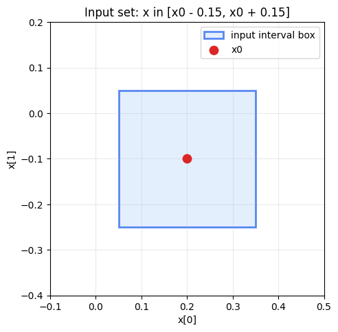
Visualising the Input Box
The IBP input set is an axis-aligned box. In two dimensions, it is easy to draw directly.
def plot_input_box(center: np.ndarray, eps: float) -> None:
    fig, ax = plt.subplots(figsize=(5, 5))
    lower, upper = center - eps, center + eps
    ax.add_patch(
        Rectangle(lower, upper[0] - lower[0], upper[1] - lower[1], facecolor="tab:blue", alpha=0.2, edgecolor="tab:blue", linewidth=2, label="input interval box")
    )
    ax.scatter(*center, color="tab:red", zorder=3, label="x0")
    ax.set_xlim(lower[0] - 0.2, upper[0] + 0.2)
    ax.set_ylim(lower[1] - 0.2, upper[1] + 0.2)
    ax.set_xlabel("x[0]")
    ax.set_ylabel("x[1]")
    ax.set_title(f"Input set: x in [x0 - {eps}, x0 + {eps}]")
    ax.legend()
    ax.grid(True, alpha=0.3)
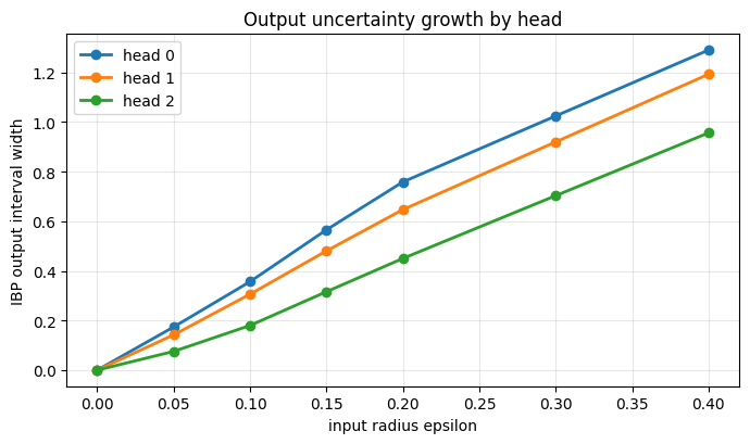
Output Intervals for Increasing Input Uncertainty
As epsilon grows, the input box grows. IBP propagates the larger uncertainty through the same network, so the output intervals generally widen. The next plot compares output intervals for several epsilon values.
eps_values = np.array([0.00, 0.05, 0.10, 0.15, 0.20, 0.30, 0.40])
records = []

for eps in eps_values:
    eps_bounds = ibp_network(net, x0, float(eps))
    lower, upper = eps_bounds["output"]
    records.append((eps, lower, upper, upper - lower))
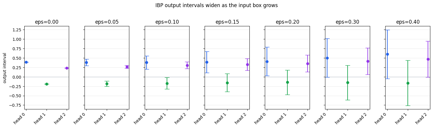
The interval bars are certified enclosures. They are allowed to be wider than the sampled output range, but the sampled range should not escape them.
Checking All Epsilons Against Samples
A sampling check is not a proof, but it is a useful sanity check for the implementation. The proof comes from the interval arithmetic rules above; the samples merely help catch coding mistakes.
for eps in eps_values:
    eps_bounds = ibp_network(net, x0, float(eps))
    input_lower, input_upper = eps_bounds["input"]
    output_lower, output_upper = eps_bounds["output"]
    sample_lower, sample_upper, _ = sampled_output_range(net, input_lower, input_upper, n=30_000)

    assert np.all(sample_lower >= output_lower - tol), f"sample lower escaped for eps={eps}"
    assert np.all(sample_upper <= output_upper + tol), f"sample upper escaped for eps={eps}"
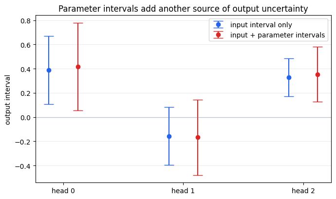
IBP With Parameter Intervals
So far, only the input was uncertain. IBP can also bound outputs when the neural network parameters are uncertain. This is useful when weights are quantized, rounded, estimated from data, perturbed by hardware noise, or represented by confidence intervals.
Suppose each weight and bias belongs to an interval:
\[W_{ij} \in [\ell^W_{ij}, u^W_{ij}], \qquad b_i \in [\ell^b_i, u^b_i].\]For an affine layer z = W x + b, each term is now a product of two intervals. For one scalar product,
The affine output interval is the sum of those product intervals plus the bias interval. If the input is exact, set lower == upper == x0; if both inputs and parameters are uncertain, propagate both kinds of intervals together. ReLU is handled exactly as before because it is monotone.
def interval_product(
    a_lower: np.ndarray,
    a_upper: np.ndarray,
    b_lower: np.ndarray,
    b_upper: np.ndarray,
) -> tuple[np.ndarray, np.ndarray]:
    """Elementwise interval product [a_lower, a_upper] * [b_lower, b_upper]."""
    candidates = np.stack(
        [
            a_lower * b_lower,
            a_lower * b_upper,
            a_upper * b_lower,
            a_upper * b_upper,
        ],
        axis=0,
    )
    return candidates.min(axis=0), candidates.max(axis=0)


def affine_interval_uncertain_params(
    W_lower: np.ndarray,
    W_upper: np.ndarray,
    b_lower: np.ndarray,
    b_upper: np.ndarray,
    x_lower: np.ndarray,
    x_upper: np.ndarray,
) -> tuple[np.ndarray, np.ndarray]:
    """Propagate intervals through z = W x + b when W, b, and x are intervals."""
    prod_lower, prod_upper = interval_product(
        W_lower,
        W_upper,
        x_lower[None, :],
        x_upper[None, :],
    )
    z_lower = prod_lower.sum(axis=1) + b_lower
    z_upper = prod_upper.sum(axis=1) + b_upper
    return z_lower, z_upper


def make_parameter_intervals(
    net: TinyMultiHeadNetwork,
    W1_radius: float,
    b1_radius: float,
    head_W_radius: float,
    head_b_radius: float,
) -> dict[str, tuple[np.ndarray, np.ndarray]]:
    """Create symmetric parameter intervals around the nominal network."""
    return {
        "W1": (net.W1 - W1_radius, net.W1 + W1_radius),
        "b1": (net.b1 - b1_radius, net.b1 + b1_radius),
        "W_heads": (net.W_heads - head_W_radius, net.W_heads + head_W_radius),
        "b_heads": (net.b_heads - head_b_radius, net.b_heads + head_b_radius),
    }


def ibp_network_with_parameter_intervals(
    params: dict[str, tuple[np.ndarray, np.ndarray]],
    center: np.ndarray,
    eps: float,
) -> dict[str, tuple[np.ndarray, np.ndarray]]:
    """Bound outputs when both inputs and network parameters are interval-valued."""
    input_lower = center - eps
    input_upper = center + eps
    hidden_pre_lower, hidden_pre_upper = affine_interval_uncertain_params(
        *params["W1"],
        *params["b1"],
        input_lower,
        input_upper,
    )
    hidden_lower, hidden_upper = relu_interval(hidden_pre_lower, hidden_pre_upper)
    output_lower, output_upper = affine_interval_uncertain_params(
        *params["W_heads"],
        *params["b_heads"],
        hidden_lower,
        hidden_upper,
    )
    return {
        "input": (input_lower, input_upper),
        "hidden_pre": (hidden_pre_lower, hidden_pre_upper),
        "hidden": (hidden_lower, hidden_upper),
        "output": (output_lower, output_upper),
    }


param_bounds = make_parameter_intervals(
    net,
    W1_radius=0.04,
    b1_radius=0.02,
    head_W_radius=0.035,
    head_b_radius=0.015,
)
param_bounds_exact_input = ibp_network_with_parameter_intervals(param_bounds, x0, eps=0.0)
param_bounds_input_box = ibp_network_with_parameter_intervals(param_bounds, x0, eps=epsilon)
The first parameter-interval run fixes the input at x0, so all output uncertainty comes from the weights and biases. The second run combines the same parameter intervals with the input box used earlier.
def sample_network_from_parameter_intervals(
    params: dict[str, tuple[np.ndarray, np.ndarray]],
    rng: np.random.Generator,
) -> TinyMultiHeadNetwork:
    return TinyMultiHeadNetwork(
        W1=rng.uniform(*params["W1"]),
        b1=rng.uniform(*params["b1"]),
        W_heads=rng.uniform(*params["W_heads"]),
        b_heads=rng.uniform(*params["b_heads"]),
    )


def sample_outputs_with_parameter_intervals(
    params: dict[str, tuple[np.ndarray, np.ndarray]],
    input_lower: np.ndarray,
    input_upper: np.ndarray,
    n: int = 20_000,
    seed: int = 1,
) -> np.ndarray:
    rng = np.random.default_rng(seed)
    outputs = []
    for _ in range(n):
        sampled_net = sample_network_from_parameter_intervals(params, rng)
        x = rng.uniform(input_lower, input_upper)
        outputs.append(sampled_net.forward(x))
    return np.asarray(outputs)


input_lower, input_upper = param_bounds_input_box["input"]
output_lower, output_upper = param_bounds_input_box["output"]
parameter_sampled_outputs = sample_outputs_with_parameter_intervals(param_bounds, input_lower, input_upper)
sample_lower = parameter_sampled_outputs.min(axis=0)
sample_upper = parameter_sampled_outputs.max(axis=0)

assert np.all(sample_lower >= output_lower - tol)
assert np.all(sample_upper <= output_upper + tol)
Related Methods
IBP is one point in a larger family of neural network bounding and verification methods. Closely related approaches include:
- Linear bound propagation / CROWN: propagates linear upper and lower relaxations rather than only scalar intervals, often giving tighter bounds.
- alpha-CROWN and branch-and-bound variants: optimize relaxations and split difficult domains to tighten certificates.
- DeepPoly, zonotopes, and abstract interpretation: track richer abstract sets so some correlations between neurons are preserved.
- Lipschitz and spectral-norm bounds: give global sensitivity certificates, usually coarser but cheap to compute.
- MILP or SMT verification: can be much tighter, sometimes exact for ReLU networks, but usually scales worse.
- Randomized smoothing: certifies robustness probabilistically by smoothing the classifier with noise rather than propagating deterministic bounds.
In practice, IBP is attractive because it is simple, differentiable, and fast enough to use during training, while tighter methods are often used for final verification or for harder examples.
What To Notice
- IBP is fast because each layer is processed once with vectorized interval arithmetic.
- The method is sound for affine layers and monotone activations such as ReLU.
- Wider input boxes and wider parameter intervals both tend to produce wider output intervals.
- Parameter intervals require product-interval arithmetic because terms like
w * xmay have uncertainty in both factors. - The bounds may be conservative because correlations between neurons and parameters are not tracked. For example, two hidden units may not be able to reach their worst-case values at the same concrete input, but interval arithmetic treats them independently.
The next natural step is to take this machinery to an actual RL environment — certifying that a trained policy’s action stays within a safe set for every state in some neighbourhood (and under some amount of parameter uncertainty), for example on MountainCar. That worked example is coming in a future post.